12.2 Crest level design#
12.2.1 Hydraulic boundary conditions#
The relevant hydraulic boundary conditions for ‘overflowing’ and ‘wave overtopping’ are water levels and waves (height and period or spectrum). Preferably the design boundary conditions are calculated using a probabilistic method based on design formulae and sufficient statistical information such as water level distributions. Given a target reliability the probabilistic method yields so-called design values for water level, wave height and wave period for a specific geometry of the dike and a failure mechanism. In the Netherlands models like HYDRA-NL (design) and/or RINGTOETS (safety assessment) are based on a probabilistic method (see Chapter 10 for more information).
Using the more traditional flood protection methods the design water levels, wave heights and wave periods are related to fixed return periods and based on a statistic analysis from field data and/or computed data. Based on this analysis a 100-year water level and/or a 10-year wave height can be calculated. Depending on the data available a multi-variate analysis may give information on conditional probability distribution of waves at certain water levels. Chapter 4 of these Lecture Notes shows more information. If sufficient data of water levels at a certain location is available, this data can be used to determine a statistical distribution of water levels. However, these earlier water levels include the effects of tide, the spring/neap tides, storm surges at sea, wind setup at lakes and/or flood plains, seiches (caused by air pressure effects) or other oscillations, natural changes in bathymetry or morphology, man made projects and climate change. To determine an accurate statistical distribution these effects have to be accounted for to create a homogeneous set of data.
For river systems the data may be related to the recorded water levels and/or discharges at a fixed location. In the Netherlands the water levels and discharges at Lobith (Rhine) or Borgharen (Meuse) are used. An improvement on this statistical approach is the introduction of precipitation-runoff-discharge models. These models generate artificial discharges based on (expected) precipitation statistics. The precipitation statistics are in most case readily available, leading to more accurate discharge statistics for locations without a long history of recorded data.
For coastal systems again the data may be related to the recorded water levels at fixed locations. In the Netherland the water levels at Hoek van Holland, Vlissingen, Ijmuiden, Den Helder, Harlingen and Delfzijl are often used. In some cases data is available for a period of more than 100 years. In this case, mathematical models have been introduced as well. For example, a meteorological model predict water levels and wave height along the Dutch coast for a certain weather situation. The advantage of introducing mathematical models is not only the use of meteorological data, but it also gives a correlation between water levels and other hydraulic boundary conditions, such as waves.
Considering that a flood protection structure will be designed to provide flood protection for a number of decades ahead future climate change effects on water levels need to be accounted for. The past experience in the Netherlands with sea level rise indicate rise of 20 cm per century, but for the future a number of scenarios have been developed within the Delta programme (Delta programme, 2014). The effects of these scenarios range from to 35 or 85 cm for 2100. For design purposes the upper scenario is used (2050: +0.35 meters; 2100: +0.85 meters).
Climate change also effects river discharges and this effect is often estimated at 10 to 20% in 50 to 100 years. The estimated effects of climate scenarios for the Rhine range from an additional 1,000 to 2,000 \(m^3\)/sec. Again the upper scenario is used (2050: 17,000 \(m^3\)/sec; 2100: 18,000 \(m^3\)/sec). However, in river systems the increased discharge may be affected by flooding upstream. For example, based on mathematical modelling the maximum discharge in the river Rhine at Lobith is limited to 17,500 to 18,000 \(m^3\)/sec, because the river dikes in Germany will flood. For Meuse the climate scenarios range from +2,000 \(m^3\)/sec to +6,000 \(m^3\)/sec (!!).Again the upper scenario is used (2050: 4,200 \(m^3\)/sec; 2100: 4,600 \(m^3\)/sec).
The difficulty is to decide on the climate scenario used in a design process. Again, the best thing to do is to make a full probabilistic analysis. In such an analysis the design can be tested against the various scenarios with varying lifespan for the structure. If a probabilistic analysis is not made, an educated guess can be made based on a sensitivity analysis. As a rule of thumb, the following two choices are in general sensible:
Structures with relatively high construction cost and with little adaptability are to be designed with a long lifespan (50-100 years) and a conservative climate scenario.
Adaptive structures with relatively low (re)construction costs are to be designed with a short lifespan (25-50 years) and a medium or even optimistic climate scenario.
Additional factors contributing to design water levels are wind setup and seiches (oscillations). Wind setup is usually incorporated in sea or lake level statistics (storm surge effect). However, in rivers local wind setup may be an issue in the shallow flood plains. This effect needs to be calculated separately as the water level data in rivers are often derived from discharge statistics. The wind data used to determine wave conditions can be used for wind setup too. Seiches and other forms of oscillating water levels are generally not included in water level statistics. Their effect needs to be added too, taking into account that seiches are not (fully) correlated with storms. Chapter 4 of these Lecture Notes contains more information on seiches and oscillations.
Having established the design water level (including effects of climate change and seiches) related to the required return period the next essential elements to calculate the required dike crest level are wave boundary conditions: wave height and wave period.
For a river situation the water levels (river flood) and wave conditions are not likely to be very correlated and therefore the wind generated waves may be determined based on wind statistics (speed and direction), the fetch length and water depths. For a coastal situation water levels (storm surge) and wave conditions are very much correlated. Therefore the wave statistics are related to the water levels.
As explained in chapter 4 and 6 of these Lecture Notes one should use the hydraulic conditions at the toe of the structure. The spectral wave height and period \(H_{m0}\) and \(T_{m-1,0}\) provide the most accurate prediction of run-up and overtopping, also in non-standard cases such as double-peaked spectra and (very) shallow foreshores. The HYDRA-NL computer programme provides these wave parameters. Using the spectral wave period is important if the wave spectrum shows more energy for longer periods. Also, the spectral wave period deals better with double peaked or ‘flat’ wave spectra.
If waves are calculated otherwise (such as using the Bretschneider formula for wind generated wave) a significant wave height (\(H_{s}\)) and a peak period (\(T_{p}\)) are calculated. Using these parameter requires re-fitted design formulae or the wave parameters need to be adapted. In deep water the differences are very small, but in shallow water differences may increase to 10-15%. Based on the spectral wave height it is straightforward to calculate a wave height distribution and the significant wave height []. For the failure mechanisms related to stability under wave attack (such as revetments) and for the assessment of dunes the peak period (\(T_{p}\)) is used. If the spectral period is known the value of \(T_{p}\) can be calculated easily: \(T_{p} = 1,1 \cdot T_{m-1,0}\).
12.2.2 Definition of the examples and hydraulic boundary conditions#
Example river dike#
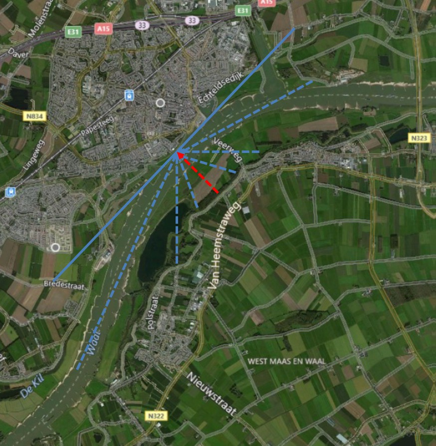
For a river dike two examples will be illustrated, using the traditional approach and the new safety standards. The location of the river dike is near Tiel on the north bank of the Waal, the main branch of the river Rhine (figure 12.23). The solid blue line shows the orientation of the dike with the normal in red (SE direction, 135°). The red and blue dashed lines indicate the various fetch lengths.
The statistical information for the water levels at this location is shown in Tab:Hydr_bc_riverdike. The traditional approach at this location featured a safety standard of 1/1250 per year. As an illustration, the return periods used for the German safety standards (1/100 per year for the upper river and 1/200 per year for the lower river) are shown too. However, it must be emphasized that the design rules in Germany are different from the Dutch rules.
The wave loads are wind generated and calculated using a standard wind field (1 hour average) and the Bretschneider prediction formula. It is assumed that the waves will fully developed within an hour. This is reasonable, given the maximum fetch lengths in the river area. The wave height and wave period can be calculated using a wind speed and the water depth in the foreshore (5 meters in this example). For the shorter return periods the water level is obviously lower (1 meters in this example) and therefore the wave loads are somewhat lower too. The effects of climate change in 2100 is also shown in Tab:Hydr_bc_riverdike by the figures between brackets.
The new safety standard for this location is 1/30,000 per year. This probability is used to derive the water levels for geotechnical and piping design. Using the standard design formulae the target probability for ‘overflowing’ and ‘overtopping’ is based on a value of \(\omega\) of 24% and a length-effect N of 1. The target probability is 1/125,000 per year. Using the model HYDRA-NL the design conditions for this location, failure mechanism (wave overtopping) and dike geometry are calculated and shown in Tab:Hydr_bc_riverdike. As explained in Subsec:Der_designvalues, HYDRA-NL performs a full probabilistic analysis for the hydraulic loads and the presented combination of water level, wave height and wave period is the design point. This design point is valid only for wave overtopping (5 l/m/s). For other overtopping rates and failure mechanisms other design points need to be calculated. For example, for the design of a revetment various design points are needed to calculate the required revetment at various water levels.
Table 12.1: Hydraulic boundary conditions river dike example
Return period [year] |
Water level [m] |
Wave height [m] |
Wave period [s] |
|
|---|---|---|---|---|
Traditional approach |
100 |
10.1 (10.5) |
0.4 (0.4) |
2.1 (2.1) |
200 |
10.3 (10.8) |
0.4 (0.4) |
2.1 (2.1) |
|
1250 |
10.8 (11.5) |
0.4 (0.5) |
2.3 (2.5) |
|
New safety standard |
Safety standard [1/year] |
Water level [m] |
Wave height [m] |
Wave period [s] |
1/30000 |
11.4 (11.5) |
– |
– |
|
1/125000 |
11.5 (11.5) |
0.6 (1.0) |
2.7 (3.4) |
The numbers in table 12.1 show very clearly the effect of the maximum discharge of 18,000 \(m^3\)/sec. The water level is limited to MSL+11.5 meters, but the waves are not limited due to the increasing wind speeds at the smaller probabilities.
Before using the hydraulic boundary conditions the margins for statistical uncertainties need to be added. For the river area the additional margin for the water level is 0.3 meters. For the wave loads a 10% margin is added to both the wave height and wave period.
Example coastal dike#
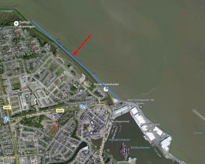
For a coastal dike also two examples will be illustrated, using the traditional approach and the new safety standards. The location of the river dike is near Delfzijl on the shores of the Wadden Sea (figure 12.24). The solid blue line shows the orientation of the dike with the normal in red (NE direction, 45°).
The statistical information for the water levels at this location is shown in table 12.2. The traditional approach at this location featured a safety standard of 1/4,000 per year. Again as an illustration, the water levels are also shown for return periods related to the German safety standards for the Wadden Sea (1/100 per year) and for the Hamburg area (1/400 per year). The waves are derived using the HYDRA-NL model. The effects of climate change is also shown in table 12.2.
The new safety standard for this location is 1/10,000 per year. This probability is used to derive the water levels for geotechnical and piping design. Using the standard design formulae the target probability for ‘overflowing’ and ‘overtopping’ is based on a value of \(\omega\) of 24% and a length-effect N of 1. The target probability is 1/41,667 per year. Using the model HYDRA-NL the design conditions for this location, failure mechanism (wave overtopping) and dike geometry are calculated and shown in table 12.2. As explained in section 10.2.4 HYDRA-NL performs a full probabilistic analysis for the hydraulic loads and the presented combination of water level, wave height and wave period is the design point. This design point is valid only for wave overtopping (5 l/m/s). For other overtopping rates and failure mechanisms other design points need to be calculated.
Table 12.2: Hydraulic boundary conditions coastal dike example
Return period [year] / Safety standard [1/year] |
Water level [m] |
Wave height [m] |
Wave period [s] |
|
|---|---|---|---|---|
Traditional approach |
100 |
5.0 (5.8) |
1.3 (1.6) |
4.0 (4.5) |
400 |
5.4 (6.2) |
1.6 (1.9) |
4.2 (4.7) |
|
4000 |
6.1 (6.9) |
1.9 (2.2) |
4.5 (5.0) |
|
New safety standard |
Safety standard [1/year] |
Water level [m] |
Wave height [m] |
Wave period [s] |
1/10000 |
6.3 (7.2) |
– |
– |
|
1/41667 |
6.3 (7.2) |
2.3 (2.6) |
4.8 (5.3) |
Before using the hydraulic boundary conditions the margins for statistical uncertainties need to be added. For the coastal area the additional margin for the water level is 0.4 meters. For the wave loads a 10% margin is added to both the wave height and wave period.
12.2.3 Calculation of the required crest level#
In chapter 5 of these Lecture Notes the processes of wave run-up and wave overtopping are described. For this section the TAW formula for overtopping (5.4) has been used (deterministic version). In the traditional approach the goal of the design is to calculate a required freeboard to limit the wave overtopping discharge and to keep the inner slope safe from erosion eventually leading to a dike breach. A typical critical overtopping discharge in the traditional approach ranges from 0.1 l/m/s to 5 l/m/s, depending on the quality of the inner slope of the dike.
The new safety standard is related to a dike breach and allows larger overtopping discharges. Now, the maximum critical overtopping discharges range from 5 l/m/s up to 10 l/m/s, provided the inner slope is well-covered with grass or with a clay layer of at least 80 centimeters . If macro-instability and/or erosion of the inner slope can be prevented (e.g. by mild slopes or by reinforcing the inner slope) even much higher overtopping discharges can be allowed. Obviously, if very high overtopping discharges are allowed the potential consequences for the hinterland need to be assessed properly.
Table 12.3 shows the required freeboard for a critical overtopping discharge of 1 l/m/s, calculated with the TAW formula [29]](Eq:Max_simple_Ru) for overtopping and a fixed wave steepness of 4%.
Table 12.3: Required freeboard based on wave overtopping
Wave height [m] |
Cotan outer slope [-] |
|||||
|---|---|---|---|---|---|---|
2 |
3 |
4 |
5 |
8 |
||
River dikes |
||||||
0.20 |
0.31 |
0.28 |
0.20 |
0.16 |
0.09 |
|
0.50 |
1.04 |
0.94 |
0.69 |
0.54 |
0.32 |
|
0.80 |
1.88 |
1.71 |
1.25 |
0.98 |
0.59 |
|
Coastal dikes |
||||||
Wave height [m] |
Cotan outer slope [-] |
|||||
2 |
3 |
4 |
5 |
8 |
||
2.00 |
5.75 |
5.23 |
3.85 |
3.03 |
1.83 |
|
4.00 |
13.10 |
11.91 |
8.78 |
6.93 |
4.21 |
|
8.00 |
29.40 |
26.73 |
19.75 |
15.61 |
9. |
| 8.00 | 29.40 | 26.73 | 19.75 | 15.61 | 9.81 |
The results in the table 12.3 show how the required freeboard works out for river dikes (with small waves) and for sea dikes (higher waves). It also shows that river dikes may have relatively steep slopes (1:2 or 1:3). Such steep slopes are not really an option for sea dikes: gentler slopes of 1:5 or less yield more realistic freeboards. It is clear that a gentler outer slope is very effective in reducing the required freeboard. On the other hand, very mild slopes are not very like to be applied in the river area because of the large footprint required. The unrealistic options in table 12.3 are indicated in italics. Also a number of combinations yields a freeboard less than the minimum required value of 0.50 meters.
Instead of overtopping the required crest level or freeboard may be calculated using wave run-up as well. Especially in the traditional approach this method is applied very frequently because it is straight¬forward to use. The Delft formula (28) is valid for a wave steepness of 4.8% and breaker parameters less than 1.8 (common for local wind generated waves), but the TAW formula for wave run-up (28) can be applied for a wider range of circumstances. This is preferable because longer waves with more energy will run further up the slope or give a higher overtopping volume.
Table 12.4 shows the required freeboard again for a fixed wave steepness of 4.8%, calculated with the TAW formula (28) for 2% wave run-up.
Table 12.4: Required freeboard based on 2% wave run-up
Wave height [m] |
Cotan outer slope [-] |
|||||
|---|---|---|---|---|---|---|
2 |
3 |
4 |
5 |
8 |
||
River dikes |
||||||
0.20 |
0.61 |
0.55 |
0.20 |
0.41 |
0.21 |
|
0.50 |
1.53 |
1.38 |
1.03 |
0.82 |
0.52 |
|
0.80 |
2.44 |
2.20 |
1.65 |
1.32 |
0.83 |
|
Coastal dikes |
||||||
Wave height [m] |
Cotan outer slope [-] |
|||||
2 |
3 |
4 |
5 |
8 |
||
2.00 |
6.10 |
5.50 |
4.13 |
3.30 |
2.06 |
|
4.00 |
12.20 |
11.00 |
8.25 |
6.60 |
4.13 |
|
8.00 |
24.40 |
22.00 |
16.50 |
13.20 |
8.25 |
The results in the table 12.4 show on average higher required freeboards than table 12.3 for the river dikes, whilst for the coastal dikes the required freeboards are more or less similar. For these circumstances the 2% wave run-up criterion more or less equals the 1 l/m/s criterion. For the smaller waves (river area) the 2% wave run-up criterion is more strict and more or less equals the 0.1 l/m/s criterion. Again, the unrealistic options in table 12.4 are indicated in italics and a number of combinations yields a freeboard less than the minimum required value of 0.50 meters.
Example river dike#
For the river dike the design calculations are applied to the hydraulic boundary conditions of table 12.1 including the required uncertainty margins. For the geometry of the river dike two standard profiles (with an outer slope of 1:3 and 1:5) are used (no berm, no composite slopes, no shallow foreshore, no additional roughness). The effect of climate change is shown between brackets. For the traditional approach a critical overtopping discharge of 0.1 l/m/s/ is used. For the new safety standard 5 l/m/s is used. The results are shown in table 12.5.
Table 12.5: Required crest levels river dike example
Return period [year] / [1/year] |
Crest level 1:3 [m] |
Crest level 1:5 [m] |
|
|---|---|---|---|
Traditional approach |
100 |
10.9 (11.3) |
10.6 (11.0) |
200 |
11.2 (11.6) |
10.9 (11.3) |
|
1250 |
11.7 (12.4) |
11.4 (12.0) |
|
New safety standard |
Return period [1/year] |
Crest level 1:3 [m] |
Crest level 1:5 [m] |
1/125000 |
12.1 (12.4) |
11.9 (12.1) |
The results of table 12.5 show that the effect of a milder slope for the river dike is rather small, especially if larger overtopping rates are allowed (new safety standard). The effect of the new, stricter safety standard is not fully compensated by the larger overtopping rate. But for 2100 the difference between the new standard and the traditional approach diminishes about 10 centimeters. That is largely due to the maximum Rhine discharge of 18,000 \(m^3/sec\) that has been used in the calculations. The effect of climate change remains fairly constant.
Example coastal dike#
For the coastal dike the design calculations are applied to the hydraulic boundary conditions of table 12.2including the required uncertainty margins. For the geometry of the coastal dike two standard profiles with an outer slope of 1:5, with and without a berm (10 meters wide at a level of MSL+7 meters) is used (no composite slopes, no shallow foreshore, no additional roughness). The effect of climate change is shown between brackets. For the traditional approach a critical overtopping discharge of 1 l/m/s/ is used. For the new safety standard 10 l/m/s is used. The results are shown in table 12.6.
Table 12.6: Required crest levels coastal dike example
Return period [year] / [1/year] |
Crest level 1:5 no berm [m] |
Crest level 1:5 berm [m] |
|
|---|---|---|---|
Traditional approach |
100 |
6.9 (8.2) |
6.9 (7.8) |
400 |
7.6 (8.9) |
7.4 (8.3) |
|
4000 |
8.8 (10.1) |
8.2 (9.2) |
|
New safety standard |
Return period [1/year] |
Crest level 1:5 no berm [m] |
Crest level 1:5 berm [m] |
1/41667 |
8.9 (10.2) |
8.2 (9.5) |
The results of table 12.6 show that the crest level differences for the various return periods are much larger than for the river dike. The correlation between water level and waves causes this effect. The reducing effect of the berm become noticeable at the extreme return periods, because the berm is constructed at MSL+7 meters. The effect of the new, stricter safety standard is nearly completely compensated by the larger overtopping rate. The effect of climate change remains fairly constant.
12.2.4 Calculation of construction crest level#
From the required crest level a construction crest level can be calculated by taking into account the effects of land subsidence, consolidation of the subsoil of the dike and compaction of the dike. To design a dike for a number of decades ahead, the effects of land subsidence and consolidation are generally a significant factor to include in the construction crest level. These effects are more certain to occur than climate change.
The antipode of increased water levels through climate change is land (and therefore dike) subsidence. A number of factors may contribute to a subsiding dike:
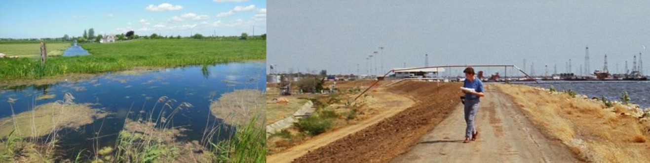
Polder drainage (figure 12.25 left): a serious problems for e.g. Dutch polders where continuous pumping for centuries has led to significant land subsidence. In the Waterland region, north of Amsterdam, this land subsidence amounts 30 to 80 cm in 100 years. Often the dike itself may experience less subsidence, since the soil under the dike is more consolidated.
Extraction of groundwater or oil (figure 12.25 right): extreme examples are Jakarta (10 cm per year as a result of massive private wells for industry and drinking water) or Lago de Maracaibo in Venezuela (as a result of oil exploration from the lake bottom and from the land, some 5 meters subsidence in the latest 30 years on top of 4 meters subsidence between 1920 and 1985).
Tectonic movement and tilt: In addition to the above mentioned more important features, geological activity may lead to relatively reduced (or increased) dike levels. In highly seismic active areas, earthquakes may lead to more serious changes of large regions, changing the general reference level considerably, meters. This has e.g. been observed in Río Cauca basin in Colombia, but also for the west coast of Sumatra after the 2004 earthquake leading to the Christmas tsunami.
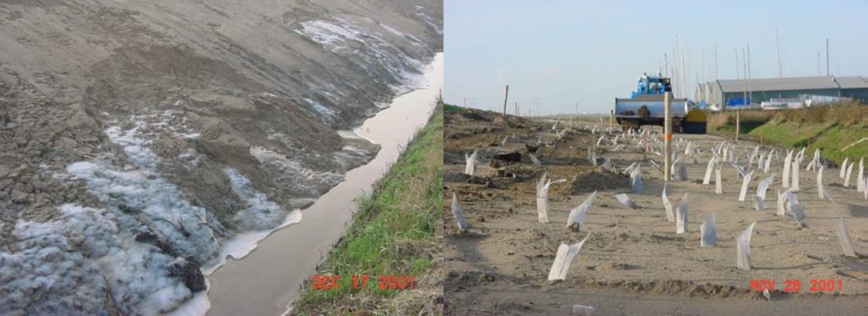
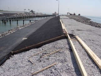
After the construction of a dike the subsoil will not have consolidated yet. The groundwater will be in a situation of overpressure and slowly drain from the less permeable layers: this process is called consolidation. This will cause dike settlement. Especially in weak soils this factor can be significant and should be accounted for in the construction height. This factor is also important for the geotechnical stability during or shortly after construction. Figure 12.26 (left) shows groundwater flowing out of a slope under pressure of the newly built dike. Because of the freezing weather the groundwater gets frozen and stay very well visible. Figure 12.26 (right) shows the vertical drainage flaps which are used to enhance consolidation.
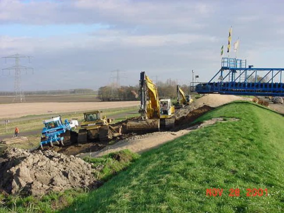
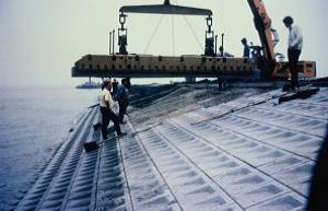
Compaction of the dike body itself should be done properly during construction. Contractors are usually required to fill the dike body with small layers of 40 cm and compact them with bulldozers to a fixed Proctor rate of e.g. 97%. With modern equipment dike compaction after construction is virtually negligible. Figure 12.27 shows soil being brought into the dike body from a conveyor belt. This soil is being spread into relatively thin layers and being compacted by two bulldozers in alternating directions.
12.2.5 Options for optimization#
Calculating the crest level is an important step in the technical design process. The first iteration as performed in the previous section may lead to complications. These complications can be technical (geotechnical stability), but also there may be restrictions like a maximum footprint or a maximum crest level. Reduction of wave overtopping or wave run-up is then an option to design a lower crest. Starting at the hydraulic conditions a number of options is available.
Foreshore#
The wave action on the outer slope of the dike can be limited by reducing the waves. This can be done by raising the foreshore or by using vegetation. By raising the foreshore the waves will become depth limited and if the foreshore is wide enough to allow breaking of the larger waves the maximum waves will reduce to 0,55 of the water depth (during storm conditions obviously).
The effect of a shallow foreshore can be enhanced by using vegetation. In the Netherlands along the rivers willow trees can be used. But in tropical regions mangroves or salt water marshes (New Orleans) are able to reduce the impact of storm surges by breaking the waves.
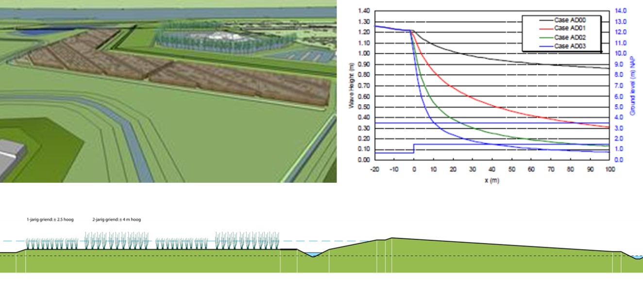
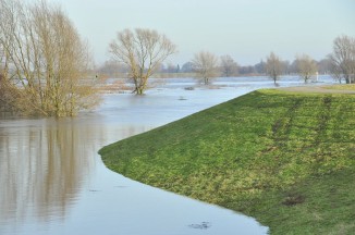
An excellent example is a project in the polder Noordwaard near Werkendam. This project is part of Room for the River and during river floods a significant part of this polder will be flooded. The other parts are protected by using mounds (terpen in Dutch) or by constructing dikes. Fort Steurgat is an old fortress changed into a residential area and a new dike has to be constructed in front of the fort. There was public opposition against the traditional design of the dike. It was considered too high, blocking the view from the Fort but also contrasting with landscape by the use of concrete revetments. A solution was found by a lower, hybrid dike without revetments and with willow trees reducing the waves. This dike is integrated in the landscape and it is expected that the new design will add to recreational value of the area for local residents.
This was possible by reducing the wave loads. During a flood the design wave Hs is 1 to 1.2 meters. That is due to the long fetch (10 km) and the considerable water depth (3 m) under the design conditions. From field and laboratory research it has become clear that vegetation can be an effective means of wave reduction (\cite{Coops.H._et.al.},\cite{Mendez2004}, [] or []). In the final design a continuous willow tree plantation in front of the dike provides 80% reduction of incoming wave height under 1/2000 per year storm conditions. This allows the dike crest to be 1 meter lower than in the traditional design. An a simple clay cover is sufficient to resist the remaining wave attack. The willow plantation is inspired by the centuries old tradition of willow culture for the production of brushwood, which is typical of this region. Thanks to this know-how, tree vitality can be guaranteed and long-term maintenance of the plantation can be defined and budgeted.
A number of design aspects are relevant:
The integrated dike including the willow plantation has a wider footprint than the traditional dike. The width of the willow plantation needed is quite substantial. This may interfere with the required discharge capacity of the river. Furthermore, it needs to fit into existing plans for nature- and landscape development or even better, an integrated plan for the flood plain.
The design features a willow tree plantation. This is beyond the expertise of traditional dike engineers and requires expert input of biologists. Biologists need to be involved during the design and construction of the dike. Planning of dike construction is more complex compared to a traditional design as a sufficiently dense tree plantation takes time to grow (3-4 years).
Nearly all Building with Nature measures require more and complicated maintenance. The willow plantation has to be maintained yearly to guarantee sufficient density and tree health.
Research [] demonstrated that the main wave reduction is already realised in the first 20 m of the forest, which means that future designs could possibly have smaller dimensions (see figure 12.28, top-right).
Applying an innovation like this requires sound documentation, especially for future safety assessments [].
Based on the traditional design approach the design calculations for (one section of) Fort Steurgat are shown (adapted from Dekker and de Vries, 2009). The overtopping criterion used is 2 l/m/s, based on the very mild inner slope. The outer slope is 1:5 and the (positive) effect of the vegetation on the wave period is neglected.
Table 12.7: Design calculations for Fort Steurgat
Return period [year] |
Water level [m + MSL] |
Wave height [m] |
Wave period [s] |
|
|---|---|---|---|---|
Boundary conditions |
2000 |
3.4 |
1.1 |
4.4 |
Effect climate change |
+0.15 |
– |
– |
|
Margin for uncertainty |
+0.30 |
+10% |
+10% |
|
Design Conditions |
3.85 |
1.21 |
4.84 |
Reduction wave height |
Water level [m + MSL] |
Wave height [m] |
Crest level [m + MSL] |
|
|---|---|---|---|---|
Design calculations |
0% |
3.85 |
1.21 |
5.50 |
20% |
3.85 |
0.97 |
5.25 |
|
40% |
3.85 |
0.73 |
5.00 |
|
60% |
3.85 |
0.48 |
4.70 |
|
80% |
3.85 |
0.24 |
4.35 |
The results confirm a reduction of the required crest level from 5.50 to 4.35 meters above MSL (based on a minimum freeboard of 0.5 meters).
Outer slope#
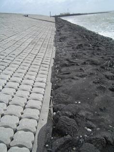
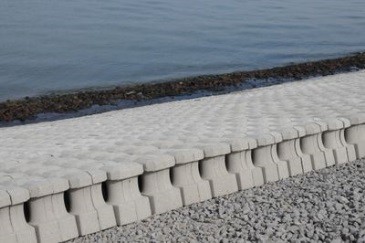
Wave overtopping or wave run-up can be reduced by applying milder outer slopes, but also by using a type of revetment with a greater roughness than grass of asphalt. The effect of reducing the outer slope angle reduction is already incorporated in the design formulae.
The effect of a rougher slope revetment than the standard grass or asphalt is that the energy of the waves running up the slope is being absorbed. When a wave runs up the slope, it dissipates energy. Rougher revetments absorb more wave energy, resulting in reduced overtopping and/or run up. revetments are expensive elements and are usually avoided where possible. But if a revetment is already necessary, applying a certain roughness will help to reduce the overtopping and/or run-up. Also maintenance, operational and environmental issues may be important considerations for the selection of one type or another.
The application of the reduction factor \(\gamma_{R}\) is described in Chapter 6 of these Lecture Notes. Structural design of revetments is described in Chapter 9 of these Lecture Notes.
Some considerations for selecting a type of revetment:
Smooth surfaces (asphalt, grass) are easily accessible, where necessary for maintenance or secondary functions of the dike. Grass slopes can be used as grazing ground for sheep. Larger cattle will damage the grass slopes.
Grass will need maintenance and careful inspection. Mowing, grazing and treating bare spots; the fact that it concerns natural material requires attention. Rip-rap requires often little maintenance, but at places with a lot of debris (plants, branches, waste), maintenance can become a heavy burden.
In case of damage after a flood or storm, inspection is required to make sure that the revetment will regain its proper condition for the next event. Repair of grass, asphalt is different, but still relatively easy, although heavy equipment may be required. Repair of rip rap may be more difficult already: often with equipment from the water side. Repair of pitched stone is usually more difficult, requires careful approach.
Depending on the other functions of the dike, different options may be selected. Accessibility or direct use for cattle, fishermen, recreation or natural life need to be considered. Esthetical aspects may also play a certain role.
|
Stone mastic asphalt, sand asphalt; γR = 1.00 open asphalt; γR = 0.90 |
 |
 |
Grass; γR = 1.00 |
|
Concrete blocks, like armourflex and haringman, γR = 0.90 |
 |
 |
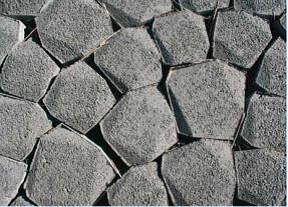
Pitched basalt; γR = 0.95 |
|
Asphalt or concrete impregnated rock; γR = 0.80, Pattern impregnated; γR = 0.70 |
 |
 |
Pitched basalton, Hydroblock, Pit polygon; γR = 0.90 |
|
Elastocoast; γR = 0.55–0.77 |
 |
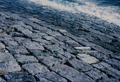 |
Rough stone with relatively much open space, example pitched natural stone (Doornik); γR = 0.75 |
|
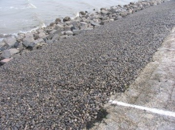
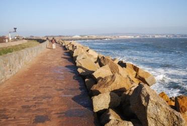
Armour rock, rip rap; γR = 0.55 (2 layer), Coarse gravel; γR = 0.70 |
 |
 |
Pitched Hill block; γR = 0.71–0.78 |
Berm#
Another option, often applied for higher, but not too long waves (lake and coastal dikes) is to interrupt the seaside slope with a smoother, almost horizontal section, the – wave breaking – berm. Especially for coastal dikes, wave energy reduction is an important issue. A horizontal section in the sea-side slope will help to break the waves. In many cases, such a horizontal section will also serve as an inspection and maintenance road. The effectivity and efficiency of the berm is a design consideration that has two main aspects:
Effectivity of wave reduction \(\rightarrow\) reduction crest level \(\rightarrow\) reduction footprint;
Reduction of dike construction costs, because the less dike material to be used with the same crest level.
The application of the reduction factor \(\gamma_{B}\) is described in Chapter 6 of these Lecture Notes. Tab:gammab_red shows the relative effectivity of a berm for different waves in practice. It shows that for coastal conditions with longer waves (10 seconds) the maximum reduction of 40% requires very wide berms (80 meters). From a more practical point of view a reduction of 5 to 10% is more realistic, considering that a maintenance road serving as a berm is about 10 meters wide. For shorter waves obviously the similar berm becomes more effective. However, including wider berms in the design may be efficient for reducing the total volume of the dike and possible for combining functions such as recreation on the outer slope.
When designing combined slopes or relatively high-lying berms, a check must be made as to whether the calculated wave run-up level does actually reach the front of the (upper) berm. This check must take place when taking into account any influence from roughness elements, angled incoming waves and the lower lying berms already taken into account. Combining more than one berm in one dike profile means that the reduction factors must then be combined from low to high, to be determined with a minimum of 0.6. If the collective berm width is (much) greater than \(0.25*L_{0}\), then the formulae of Ch:Overtopping; are not applicable.
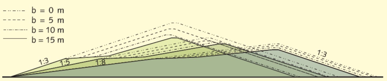
In addition to the reduction of wave overtopping and/or wave run-up the effect of a berm can be a significant reduction of the volume of the dike, as illustrated Fig:berm-effect. Especially for coastal or estuarine dikes the effects of a berm can be significant. The effect of a berm on the total volume reduces with milder slopes, but applying milder slopes may lead to less or lighter revetments. An overall optimization needs to be done based on costs.
Vertical wall#
To reduce wave overtopping a vertical wall can be applied. Although the Dutch experiences with this type of structure were not very good Subsec:Vertical_walls, vertical walls are applied in many places.
Acceptable overtopping discharge#
In the Netherlands dikes have been designed at relatively low wave-overtopping rates in the last decades: 0.1 or 1 l/s/m. These overtopping values stand for a virtually damage-free survival of the design conditions of the dike. If the land-side slope can handle the erosion and the hinterland the total overtopping volume during a flood or storm, lower dikes may be considered as an option. The effects of such an approach can be calculated using the formulae in Ch:Overtopping of these Lecture Notes. It must be emphasized that according to the new safety standards a higher overtopping discharge (5 to 10 l/m/s) is to be used anyway since the dike is expected to breach during design conditions.
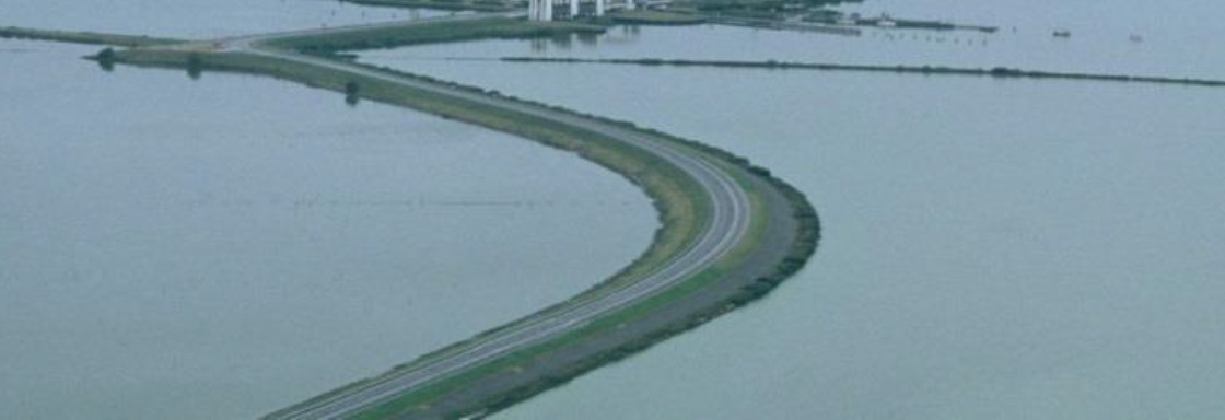
Examples of applying increased overtopping discharges in the Netherlands are the dams like Afsluitdijk and Houtribdijk. A high wave-overtopping rate is likely to be chosen, since the slopes on both sides are protected anyway and the water bodies on either side is capable of storing the total overtopping volume.
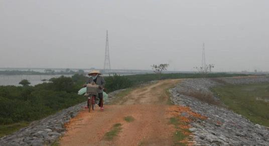
Another striking example can be found in countries with uneven spread of rainfall and river levels over the seasons. Vietnam is a good example where the wet monsoon gives virtually unmanageable floods. In the context of Vietnam these floods are allowed to overflow the dikes and the agricultural flood plains behind, a bit comparable to the flood plains of the Dutch rivers. In the dryer season, the land needs to be used for agricultural purposes and a dike needs to keep the land free from the lower river floods. These dikes will however overflow every year in the late wet season after securing the latest crop.
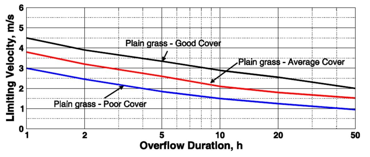
Designing such dikes is based on overflow and if geotechnical failure (following infiltration) can be prevented much higher discharges (as described in Subsec:Distr_overtop_vol) can be applied. The quality of the grass cover and the duration of the overflow (time to fill the area behind the dikes) are the governing parameters [] for grass dikes. For dikes with revetments as shown in Fig:limit_velo_overflow obviously higher velocities can be tolerated.